Python qutip用法(举例介绍)

一、N原子系综自旋概率分布

1from qutip import *
2import numpy as np
3import matplotlib.pyplot as plt
4
5n=2#原子数
6j = n//2
7psi0 = spin_coherent(j, np.pi/3, 0)#设置系统的初态为自旋相干态
8
9Jp=destroy(2*j+1).dag()#升算符
10J_=destroy(2*j+1)#降算符
11Jz=(Jp*J_-J_*Jp)/2#Jz
12
13H=Jz**2#系统的哈密顿量
14
15tlist=np.linspace(0,3,100)#时间列表
16result=mesolve(H,psi0,tlist)#态随时间的演化
17
18theta=np.linspace(0, np.pi, 50)
19phi=np.linspace(0, 2*np.pi, 50)
20
21#分别计算四个状态下的 husimi q函数
22Q1, THETA1, PHI1 = spin_q_function(result.states[0], theta, phi)
23Q2, THETA2, PHI2 = spin_q_function(result.states[30], theta, phi)
24Q3, THETA3, PHI3 = spin_q_function(result.states[60], theta, phi)
25Q4, THETA4, PHI4 = spin_q_function(result.states[90], theta, phi)
26
27#在四个子图中分别画出四个状态下的husimi q函数
28fig = plt.figure(dpi=150,constrained_layout=1)
29ax1 = fig.add_subplot(221,projection='3d')
30ax2 = fig.add_subplot(222,projection='3d')
31ax3 = fig.add_subplot(223,projection='3d')
32ax4 = fig.add_subplot(224,projection='3d')
33
34plot_spin_distribution_3d(Q1, THETA1, PHI1,fig=fig,ax=ax1)
35plot_spin_distribution_3d(Q2, THETA2, PHI2,fig=fig,ax=ax2)
36plot_spin_distribution_3d(Q3, THETA3, PHI3,fig=fig,ax=ax3)
37plot_spin_distribution_3d(Q4, THETA4, PHI4,fig=fig,ax=ax4)
38
39for ax in [ax1,ax2,ax3,ax4]:
40    ax.view_init(0.5*np.pi, 0)
41    ax.axis('off')#不显示坐标轴
42
43fig.show()

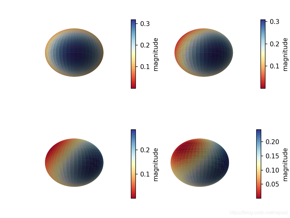
运行结果：

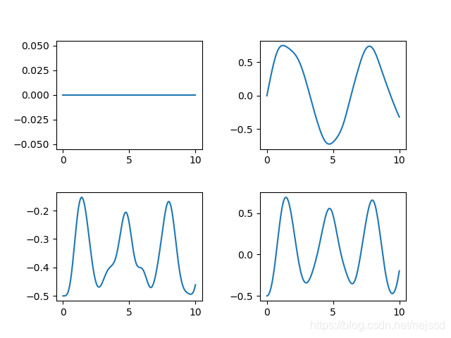
二、原子与光场相互作用

1from qutip import *
2import numpy as np
3import matplotlib.pyplot as plt
4
5alpha=1#相干光的参数alpha
6n=2#原子数
7j = n/2
8
9psi0 = tensor(coherent(10,alpha),spin_coherent(j, 0, 0))#设置系统的初态
10
11a=destroy(10)#光场的湮灭算符
12a_plus=a.dag()#光场的产生算符
13Jp=destroy(n+1).dag()#原子的升算符
14J_=destroy(n+1)#原子的降算符
15Jx=(Jp+J_)/2#原子的Jx算符
16Jy=(Jp-J_)/(2j)#原子的Jy算符,这里的j是虚数单位
17Jz=(Jp*J_-J_*Jp)/2#原子的Jz算符
18
19H=tensor(a,Jp)+tensor(a_plus,J_)#系统的哈密顿量
20tlist=np.linspace(0,10,1000)#时间列表
21result=mesolve(H,psi0,tlist)#态随时间的演化
22
23fig=plt.figure()
24ax1 = fig.add_subplot(221)
25ax2 = fig.add_subplot(222)
26ax3 = fig.add_subplot(223)
27ax4 = fig.add_subplot(224)
28
29ax1.plot(tlist,expect(tensor(qeye(10),Jx),result.states))#Jx的平均值随时间变化图
30ax2.plot(tlist,expect(tensor(qeye(10),Jy),result.states))#Jy的平均值随时间变化图
31ax3.plot(tlist,expect(tensor(qeye(10),Jz),result.states))#Jz的平均值随时间变化图
32ax4.plot(tlist,expect(tensor(qeye(10),Jx**2+Jy**2+Jz*2),result.states))#J平方的平均值随时间变化图
33
34fig.subplots_adjust(top=None,bottom=None,left=None,right=None,wspace=0.4,hspace=0.4)#设置子图间距
35fig.show()

运行结果：